Bank Marketing Campaign Data Analysis

This notebook is based on a case study that focuses on cleaning and preparing bank marketing campaign data for use in a PostgreSQL database. This analysis aims to make the data suitable for database operations, which often require data to be in a tidy format.

Introduction

Personal loans represent a significant revenue stream for banks. With typical interest rates around 10% for a two-year loan in the UK, the potential earnings are substantial. In September 2022 alone, UK consumers borrowed approximately £1.5 billion, translating to roughly £300 million in interest for banks over the loan period.

Our task is to assist a bank by cleaning the data collected from a recent marketing campaign aimed at encouraging customers to take out personal loans. As the bank plans to conduct future campaigns, ensuring the data conforms to a specific structure and data types is crucial. This cleaned data will then be used to set up a PostgreSQL database, facilitating data storage and easy import from current and future campaigns.

I have been provided with a CSV file named “bank_marketing.csv”, which requires cleaning, reformatting, and splitting into three distinct CSV files, as outlined below:

Output Files and Requirements

client.csv

Column	Data Type	Description	Cleaning Requirements
client_id	integer	Client ID	N/A
age	integer	Client’s age in years	N/A
job	object	Client’s type of job	Change “.” to “_”
marital	object	Client’s marital status	N/A
education	object	Client’s level of education	Change “.” to “_” and “unknown” to np.NaN
credit_default	boolean	Whether client’s credit is in default	Convert to boolean data type: True if “yes”, otherwise False (0).
mortgage	boolean	Whether client has existing mortgage	Convert to boolean data type: True if “yes”, otherwise False (0).

campaign.csv

Column	Data Type	Description	Cleaning Requirements
client_id	integer	Client ID	N/A
number_contacts	integer	Number of contact attempts to the client in the current campaign	N/A
contact_duration	integer	Last contact duration in seconds	N/A
previous_campaign_contacts	integer	Number of contact attempts in the previous campaign	N/A
previous_outcome	boolean	Outcome of the previous campaign	Convert to boolean data type: True if “success”, otherwise False (0).
campaign_outcome	boolean	Outcome of the current campaign	Convert to boolean data type: True if “yes”, otherwise False (0).
last_contact_date	datetime	Last date the client was contacted	Create from a combination of day, month, and a newly created year column (value 2022); Format = “YYYY-MM-DD”

economics.csv

Column	Data Type	Description	Cleaning Requirements
client_id	integer	Client ID	N/A
cons_price_idx	float	Consumer price index (monthly indicator)	N/A
euribor_three_months	float	Euro Interbank Offered Rate (EURIBOR) three-month rate (daily indicator)	N/A

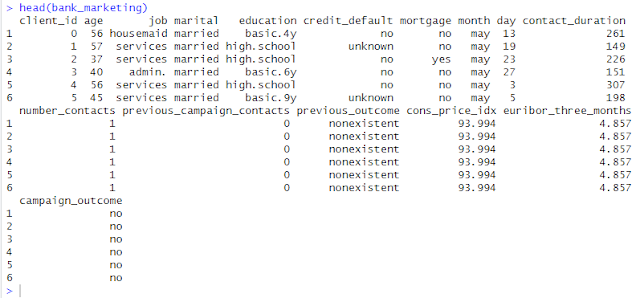
(Head of original bank_marketing.csv file)

I’m using Python and Visual Studio Code for cleaning, reformatting, and splitting into three distinct CSV files. I’m also using RStudio to view the new datasets.

Let’s Begin with Python

I’ll be using the Pandas and NumPy libraries in Python to tackle this data cleaning and transformation task.

import pandas as pd
import numpy as np

# 1. Read the CSV file
try:
    df = pd.read_csv("bank_marketing.csv")
except FileNotFoundError:
    print("Error: bank_marketing.csv not found. Make sure it's in the same directory as your Python script.")
    exit()

# Display the first 5 rows of the original dataframe
print("Original Data (First 5 Rows):")
print(df.head().to_markdown(index=False, numalign="left", stralign="left"))

Original Data (First 5 Rows):
| client_id   | age   | job       | marital   | education   | credit_default   | mortgage   | month   | day   | contact_duration   | number_contacts   | previous_campaign_contacts   | previous_outcome   | cons_price_idx   | euribor_three_months   | campaign_outcome   |
|:------------|:------|:----------|:----------|:------------|:-----------------|:-----------|:--------|:------|:-------------------|:------------------|:-----------------------------|:-------------------|:-----------------|:-----------------------|:-------------------|
| 0           | 56    | housemaid | married   | basic.4y    | no               | no         | may     | 13    | 261                | 1                 | 0                            | nonexistent        | 93.994           | 4.857                  | no                 |
| 1           | 57    | services  | married   | high.school | unknown          | no         | may     | 19    | 149                | 1                 | 0                            | nonexistent        | 93.994           | 4.857                  | no                 |
| 2           | 37    | services  | married   | high.school | no               | yes        | may     | 23    | 226                | 1                 | 0                            | nonexistent        | 93.994           | 4.857                  | no                 |
| 3           | 40    | admin.    | married   | basic.6y    | no               | no         | may     | 27    | 151                | 1                 | 0                            | nonexistent        | 93.994           | 4.857                  | no                 |
| 4           | 56    | services  | married   | high.school | no               | no         | may     | 3     | 307                | 1                 | 0                            | nonexistent        | 93.994           | 4.857                  | no                 |

Explanation:

import pandas as pd: This line imports the Pandas library, a cornerstone for data manipulation and analysis in Python. I assign it the alias pd for concise referencing. Pandas introduces powerful data structures like DataFrames (tabular data) and Series (one-dimensional data), making data cleaning, transformation, analysis, and visualization efficient. If you’re dealing with structured data similar to tables or spreadsheets, Pandas will become an indispensable tool.

import numpy as np: This line imports the NumPy library, the fundamental package for numerical computation in Python. Think of it as the bedrock for high-performance operations on arrays and matrices. NumPy provides efficient multidimensional array objects and a suite of tools for working with these arrays, making mathematical and logical operations incredibly fast and straightforward, especially when handling large datasets.

The try-except block gracefully handles the scenario where the “bank_marketing.csv” file is not found in the expected location. This prevents the program from crashing and provides a user-friendly error message to guide the user.

df = pd.read_csv(“bank_marketing.csv”): This function from Pandas reads the data from the specified CSV file and creates a DataFrame named df. A DataFrame is a two-dimensional labeled data structure with columns of potentially different types, akin to a spreadsheet or an SQL table.

Cleaning and Transforming Data for client.csv Now, let’s focus on extracting and cleaning the data required for the client.csv file.

# 2. Data Cleaning and Transformation for client.csv
client_df = pd.DataFrame()
client_df['client_id'] = df['client_id']
client_df['age'] = df['age']
client_df['job'] = df['job'].str.replace('.', '_')
client_df['marital'] = df['marital']
client_df['education'] = df['education'].str.replace('.', '_').replace('unknown', np.nan)
client_df['credit_default'] = df['credit_default'].apply(lambda x: True if x == 'yes' else False).astype(bool)
client_df['mortgage'] = df['mortgage'].apply(lambda x: True if x == 'yes' else False).astype(bool)

Explanation:

client_df = pd.DataFrame(): This line creates an empty DataFrame named client_df to store the cleaned client-related data.

client_df[‘client_id’] = df[‘client_id’] and client_df[‘age’] = df[‘age’]: These lines directly copy the client_id and age columns from the original DataFrame df to our new client_df. No cleaning is required for these columns according to the specifications.

clientdf[‘job’] = df[‘job’].str.replace(‘.’, ‘‘): Here, I access the job column in df. The .str accessor allows us to apply string methods to each element in the column. I then use .replace(‘.’, ‘‘) to replace all occurrences of a period (.) with an underscore (), fulfilling the cleaning requirement for this column.

client_df[‘marital’] = df[‘marital’]: The marital column is copied directly as no cleaning is specified.

clientdf[‘education’] = df[‘education’].str.replace(‘.’, ‘‘).replace(‘unknown’, np.nan): This line performs two cleaning operations on the education column. First, it replaces all periods with underscores. Then, it replaces all occurrences of the string “unknown” with np.nan. np.nan is a special floating-point value from the NumPy library (imported as np) that represents missing or undefined data, which is a standard way to handle missing values in Pandas.

client_df[‘credit_default’] = df[‘credit_default’].apply(lambda x: True if x == ‘yes’ else False).astype(bool): This line transforms the credit_default column to a boolean data type.

.apply(lambda x: True if x == ‘yes’ else False): This applies an anonymous function (lambda function) to each value (x) in the credit_default column. If the value is “yes”, it returns True; otherwise, it returns False.

.astype(bool): This explicitly converts the resulting column of True and False values to the boolean data type.

client_df[‘mortgage’] = df[‘mortgage’].apply(lambda x: True if x == ‘yes’ else False).astype(bool): This line performs the same boolean conversion as for the credit_default column, but for the mortgage column.

Cleaning and Transforming Data for campaign.csv Next, I’ll process the data for the campaign.csv file.

# 3. Data Cleaning and Transformation for campaign.csv
campaign_df = pd.DataFrame()
campaign_df['client_id'] = df['client_id']
campaign_df['number_contacts'] = df['number_contacts']
campaign_df['contact_duration'] = df['contact_duration']
campaign_df['previous_campaign_contacts'] = df['previous_campaign_contacts']
campaign_df['previous_outcome'] = df['previous_outcome'].apply(lambda x: True if x == 'success' else False).astype(bool)
campaign_df['campaign_outcome'] = df['campaign_outcome'].apply(lambda x: True if x == 'yes' else False).astype(bool)

# Create the 'last_contact_date' column
year = 2022
month_mapping = {'jan': 1, 'feb': 2, 'mar': 3, 'apr': 4, 'may': 5, 'jun': 6,
                 'jul': 7, 'aug': 8, 'sep': 9, 'oct': 10, 'nov': 11, 'dec': 12}
campaign_df['month_num'] = df['month'].map(month_mapping)
campaign_df['last_contact_date'] = pd.to_datetime(df['day'].astype(str) + '-' + campaign_df['month_num'].astype(str) + '-' + str(year),
                                                   format='%d-%m-%Y')
campaign_df.drop(columns=['month_num'], inplace=True) # Remove the temporary month_num column

Explanation:

Similar to client_df, an empty DataFrame campaign_df is created, and several columns (client_id, number_contacts, contact_duration, previous_campaign_contacts) are copied directly from df as they require no specific cleaning.

campaign_df[‘previous_outcome’] = df[‘previous_outcome’].apply(lambda x: True if x == ‘success’ else False).astype(bool): This line converts the previous_outcome column to boolean, mapping “success” to True (1) and all other values to False (0).

campaign_df[‘campaign_outcome’] = df[‘campaign_outcome’].apply(lambda x: True if x == ‘yes’ else False).astype(bool): This line performs the same boolean conversion for the campaign_outcome column, mapping “yes” to True (1) and other values to False (0).

Creating last_contact_date:

year = 2022: I set the year to 2022 as per the requirement.

month_mapping = {…}: A dictionary month_mapping is created to map the abbreviated month names (e.g., “jan”) to their corresponding numerical representation (e.g., 1).

campaign_df[‘month_num’] = df[‘month’].map(month_mapping): The .map() function is used to apply the month_mapping to the month column from the original DataFrame df. This creates a new column month_num containing the numerical representation of the months.

campaign_df[‘last_contact_date’] = pd.to_datetime(…): This is the core of the date creation:

df[‘day’].astype(str): Converts the day column to strings.

campaign_df[‘month_num’].astype(str): Converts the month_num column to strings.

str(year): Converts the year variable to a string.

These three string components are concatenated with hyphens (-) in between to form date strings in the format “DD-MM-YYYY”.

pd.to_datetime(…, format=’%d-%m-%Y’): This Pandas function parses the date strings according to the specified format ‘%d-%m-%Y’ and converts them into datetime objects, which are then stored in the last_contact_date column.

campaign_df.drop(columns=[‘month_num’], inplace=True): Finally, I remove the temporary month_num column as it’s no longer needed. The inplace=True argument modifies the campaign_df DataFrame directly.

Extracting Data for economics.csv Lastly, I extract the relevant data for the economics.csv file.

# 4. Data Extraction for economics.csv
economics_df = pd.DataFrame()
economics_df['client_id'] = df['client_id']
economics_df['cons_price_idx'] = df['cons_price_idx']
economics_df['euribor_three_months'] = df['euribor_three_months']

Explanation:

An empty DataFrame economics_df is created.

The client_id, cons_price_idx, and euribor_three_months columns are directly copied from the original DataFrame df to economics_df as no cleaning or transformation is required for these columns based on the specifications.

# 5. Save the DataFrames to new CSV files
client_df.to_csv("client.csv", index=False)
campaign_df.to_csv("campaign.csv", index=False)
economics_df.to_csv("economics.csv", index=False)
print("Data processing complete. Three new CSV files have been created: client.csv, campaign.csv, economics.csv")

# Display the first 5 rows of the new dataframes
print("\nFirst 5 rows of client_df:")
print(client_df.head().to_markdown(index=False, numalign="left", stralign="left"))
print("\nFirst 5 rows of campaign_df:")
print(campaign_df.head().to_markdown(index=False, numalign="left", stralign="left"))
print("\nFirst 5 rows of economics_df:")
print(economics_df.head().to_markdown(index=False, numalign="left", stralign="left"))

Data processing complete. Three new CSV files have been created: client.csv, campaign.csv, economics.csv

First 5 rows of client_df:
| client_id   | age   | job       | marital   | education   | credit_default   | mortgage   |
|:------------|:------|:----------|:----------|:------------|:-----------------|:-----------|
| 0           | 56    | housemaid | married   | basic_4y    | False            | False      |
| 1           | 57    | services  | married   | high_school | False            | False      |
| 2           | 37    | services  | married   | high_school | False            | True       |
| 3           | 40    | admin_    | married   | basic_6y    | False            | False      |
| 4           | 56    | services  | married   | high_school | False            | False      |

First 5 rows of campaign_df:
| client_id   | number_contacts   | contact_duration   | previous_campaign_contacts   | previous_outcome   | campaign_outcome   | last_contact_date   |
|:------------|:------------------|:-------------------|:-----------------------------|:-------------------|:-------------------|:--------------------|
| 0           | 1                 | 261                | 0                            | False              | False              | 2022-05-13 00:00:00 |
| 1           | 1                 | 149                | 0                            | False              | False              | 2022-05-19 00:00:00 |
| 2           | 1                 | 226                | 0                            | False              | False              | 2022-05-23 00:00:00 |
| 3           | 1                 | 151                | 0                            | False              | False              | 2022-05-27 00:00:00 |
| 4           | 1                 | 307                | 0                            | False              | False              | 2022-05-03 00:00:00 |

First 5 rows of economics_df:
| client_id   | cons_price_idx   | euribor_three_months   |
|:------------|:-----------------|:-----------------------|
| 0           | 93.994           | 4.857                  |
| 1           | 93.994           | 4.857                  |
| 2           | 93.994           | 4.857                  |
| 3           | 93.994           | 4.857                  |
| 4           | 93.994           | 4.857                  |

Explanation:

client_df.to_csv(“client.csv”, index=False): This Pandas function saves the client_df DataFrame to a CSV file named “client.csv”. The index=False argument prevents Pandas from writing the DataFrame index (row numbers) as a column in the CSV file, ensuring a clean data output.

Similar lines are used to save the campaign_df to “campaign.csv” and the economics_df to “economics.csv”.

A confirmation message is printed to the console, indicating the successful completion of the data processing and the creation of the three new CSV files.

print(client_df.head().to_markdown(index=False, numalign=”left”, stralign=”left”)): This line prints the first 5 rows of the client_df DataFrame in markdown format without the index.

print(campaign_df.head().to_markdown(index=False, numalign=”left”, stralign=”left”)): This line prints the first 5 rows of the campaign_df DataFrame in markdown format without the index.

print(economics_df.head().to_markdown(index=False, numalign=”left”, stralign=”left”)): This line prints the first 5 rows of the economics_df DataFrame in markdown format without the index.

Now, let’s add some visualizations to gain insights into the cleaned data. I’ll use histograms for numerical variables and bar plots for categorical variables in each of the three datasets.

import matplotlib.pyplot as plt
import seaborn as sns

# Set the style for the plots
sns.set(style="whitegrid")

# 6. Data Visualization

# Visualize client_df
plt.figure(figsize=(15, 10))
plt.subplot(2, 2, 1)
sns.histplot(client_df['age'], bins=20)
plt.title('Age Distribution')

plt.subplot(2, 2, 2)
sns.countplot(x='job', data=client_df)
plt.title('Job Distribution')
plt.xticks(rotation=45, ha="right")

plt.subplot(2, 2, 3)
sns.countplot(x='marital', data=client_df)
plt.title('Marital Status Distribution')

plt.subplot(2, 2, 4)
sns.countplot(x='education', data=client_df)
plt.title('Education Level Distribution')
plt.xticks(rotation=45, ha="right")
plt.tight_layout()
plt.show()

plt.figure(figsize=(15, 5))
plt.subplot(1, 2, 1)
sns.countplot(x='credit_default', data=client_df)
plt.title('Credit Default Distribution')

plt.subplot(1, 2, 2)
sns.countplot(x='mortgage', data=client_df)
plt.title('Mortgage Distribution')
plt.tight_layout()
plt.show()


# Visualize campaign_df
plt.figure(figsize=(15, 10))
plt.subplot(2, 2, 1)
sns.histplot(campaign_df['number_contacts'], bins=20)
plt.title('Number of Contacts')

plt.subplot(2, 2, 2)
sns.histplot(campaign_df['contact_duration'], bins=20)
plt.title('Contact Duration')

plt.subplot(2, 2, 3)
sns.histplot(campaign_df['previous_campaign_contacts'], bins=20)
plt.title('Previous Campaign Contacts')

plt.subplot(2, 2, 4)
sns.countplot(x='campaign_outcome', data=campaign_df)
plt.title('Campaign Outcome')
plt.tight_layout()
plt.show()

plt.figure(figsize=(8, 6))
sns.countplot(x='previous_outcome', data=campaign_df)
plt.title('Previous Campaign Outcome')
plt.tight_layout()
plt.show()


# Visualize economics_df
plt.figure(figsize=(15, 5))
plt.subplot(1, 2, 1)
sns.histplot(economics_df['cons_price_idx'], bins=20)
plt.title('Consumer Price Index Distribution')

plt.subplot(1, 2, 2)
sns.histplot(economics_df['euribor_three_months'], bins=20)
plt.title('EURIBOR Three Months Distribution')
plt.tight_layout()
plt.show()

/usr/local/lib/python3.11/dist-packages/seaborn/_oldcore.py:1119: FutureWarning: use_inf_as_na option is deprecated and will be removed in a future version. Convert inf values to NaN before operating instead.
  with pd.option_context('mode.use_inf_as_na', True):

/usr/local/lib/python3.11/dist-packages/seaborn/_oldcore.py:1119: FutureWarning: use_inf_as_na option is deprecated and will be removed in a future version. Convert inf values to NaN before operating instead.
  with pd.option_context('mode.use_inf_as_na', True):
/usr/local/lib/python3.11/dist-packages/seaborn/_oldcore.py:1119: FutureWarning: use_inf_as_na option is deprecated and will be removed in a future version. Convert inf values to NaN before operating instead.
  with pd.option_context('mode.use_inf_as_na', True):
/usr/local/lib/python3.11/dist-packages/seaborn/_oldcore.py:1119: FutureWarning: use_inf_as_na option is deprecated and will be removed in a future version. Convert inf values to NaN before operating instead.
  with pd.option_context('mode.use_inf_as_na', True):

/usr/local/lib/python3.11/dist-packages/seaborn/_oldcore.py:1119: FutureWarning: use_inf_as_na option is deprecated and will be removed in a future version. Convert inf values to NaN before operating instead.
  with pd.option_context('mode.use_inf_as_na', True):
/usr/local/lib/python3.11/dist-packages/seaborn/_oldcore.py:1119: FutureWarning: use_inf_as_na option is deprecated and will be removed in a future version. Convert inf values to NaN before operating instead.
  with pd.option_context('mode.use_inf_as_na', True):

Summary of Visualization Techniques in the Cleaning Bank Marketing Campaign notebook:

The notebook uses two primary visualization methods from the Seaborn library: histplot and countplot.

Histograms (sns.histplot)

Purpose: Histograms are used to visualize the distribution of a single numerical variable. They help in understanding how the data is spread across different ranges.

How it works:

The range of the numerical variable is divided into intervals (bins).

For each bin, the number of data points that fall within that bin is counted.

Rectangles (bars) are drawn for each bin, where the height of the bar represents the count (frequency) of data points in that bin.

Example: In the notebook, sns.histplot(client_df[‘age’], bins=20) creates a histogram of the age variable, showing how many clients fall into different age groups.

Count Plots (sns.countplot)

Purpose: Count plots are used to visualize the distribution of a single categorical variable. They display the frequency of each category.

How it works:

The unique categories in the categorical variable are identified.

The number of occurrences of each category is counted.

Bars are drawn for each category, where the height of the bar represents the count of that category.

Example: In the notebook, sns.countplot(x=’job’, data=client_df) creates a count plot of the job variable, showing the number of clients in each job category.

In essence, histplot is for numerical data, showing its distribution over a range of values, while countplot is for categorical data, showing the count of each category.

Conclusion In this case study, I successfully cleaned and transformed the bank’s marketing campaign data using Python and the Pandas library. I addressed specific data quality issues, reformatted columns to the required data types, and split the original dataset into three distinct CSV files (client.csv, campaign.csv, and economics.csv) that adhere to the bank’s specified structure.

This cleaned data is now ready to be imported into a PostgreSQL database, providing a solid foundation for analyzing the campaign’s effectiveness and for integrating data from future marketing initiatives. By establishing a consistent data structure and cleaning process, the bank can streamline its data management and gain valuable insights from its marketing efforts.

The case study and dataset used for this analysis are based on the “Project: Cleaning Bank Marketing Campaign Data” project available on DataCamp (https://www.datacamp.com/datalab/w/bfd43a29-7367-4233-a244-504e7edf2f56/edit). I want to acknowledge DataCamp for providing this valuable resource for learning and practicing data cleaning techniques.